Paying for a Meal That Had Gone Cold

Designing the kitchen

Imagine you're opening a restaurant and you want it to last. Do you build one kitchen where all the cooks work side by side, or give each cook their own station? And what does each choice cost you in the long run?

A model forecasting many related series faces the same choice. It can learn each series on its own or look across all of them. Looking across sounds better when the series are correlated. But what if the series move together and none of them predicts another? Does looking across still help? And if one series does predict another, does looking across help more as that link gets stronger?

TL;DR

Letting PatchTST look across series (channel-dependent, CD) gave no meaningful accuracy gain over forecasting each series on its own (channel-independent, CI). That held in every controlled comparison across four synthetic families.
On ECL each CD training epoch took 6.7 times as long, about 956 seconds against 143 on a T4 at the same batch size. At the finest patch size I tested, CD didn't fit on the GPU at all.
Working the maths out exactly explains why. By the 96th step ahead, the last one I scored, a series' own history already carried everything the other series could tell it. Whatever the leaders knew had faded long before then.
My default for multivariate forecasting is now channel-independent. Cross-series modelling has to earn its place on the data in front of me.

±1%mean CD vs CI gap, every controlled cell

6.7×CD epoch cost on ECL, 321 series

0cross-series information left at step 96, the last step scored

639training runs, 5 seeds per controlled cell

The kitchen choice

Our “kitchen design” questions boil down to a more practical one. If we know a series' own history, do the other series add any useful information at the horizon we're forecasting?

In multivariate forecasting there are two main design choices. The first is a channel-independent (CI) model. It shares its weights across series and forecasts each one from its own history. The second is a channel-dependent (CD) model, where information flows between series.

The model I tested is PatchTST. It cuts each series into short patches and feeds them to a Transformer as tokens. The only difference between CI and CD is what attention gets to see. In CI, each series' patches only attend to each other. In CD, every patch of every series goes into one flattened attention sequence, one shared kitchen for everything. It's the same recipe with one ingredient changed.

Channel-independent

Series 1→Encoder→Forecast 1

⋮

Series C→Encoder→Forecast C

One encoder, shared weights. Attention sees N tokens per series.

Channel-dependent, flattened

Series 1⋯Series C

↓

One sequence of C × N tokens

↓

Attention across all tokens

↓

All C forecasts

Attention sees C × N tokens at once.

The token count is simple arithmetic. A lookback of L steps cut into patches of length P at stride S gives each series

N = ⌊(L − P) / S⌋ + 1 tokens, so CI attends over N and CD over C · N

With L = 512, P = 16 and S = 8 that is 63 tokens per series. On ECL, with L = 96, it is 11 per series and 321 × 11 = 3,531 for CD, against 11 for CI. Attention work grows with the square of the sequence, so CD pays (C·N)² where CI pays C·N². A non-fused kernel also stores that score matrix: 3,531² is 12.5 million entries per head per layer, and the finest patch size I tried, P = 2 at C = 21, reaches 10,731 tokens and 115 million entries, which is where the T4 gave up.

The usual comparisons on public benchmark datasets don't settle the question either. Those datasets are observational and messy, with correlation strength, the number of series and the temporal dynamics all changing at once in ways you can't pull apart. When CD wins or loses on a benchmark, there's no way to tell what caused it.

Setting up the experiment

I built synthetic data where I could set each factor on its own and knew exactly how the data was generated. Every family is the same vector autoregression with a different transition matrix A and shock covariance Σ:

x_t = A x_t−1 + ε_t, ε_t ~ N(0, Σ), φ = 0.8 on the diagonal of A

Whatever the models could learn is in A and Σ, and only A can carry information from one series' past into another's future. Three of the four families keep it diagonal.

Family	A and Σ	What it varies	What it isolates
AR(1) grid	`A` = `φI` `Σ`_ii = 1, `Σ`_ij = `ρ`	correlation ρ (0.1, 0.5, 0.9) and series count C (7, 21, 84)	correlation with no lead-lag at all
Block covariance	`A` = `φI` `Σ`_ij = `ρ`_in inside a block of 7, 0 across	in-group ρ (0.5, 0.9) and C (21, 84)	correlated groups instead of one shared factor
Leader-follower	`A` = `φI`, plus `A`[`i`+10, `i`] = `γ` for ten pairs `Σ`_ij = 0.5	lag-1 coupling γ (0, 0.3, 0.6, 0.9) at C = 21	real lead-lag information of known strength
Patch-resolution sweep	the same `A`(`γ`) `Σ` = `σ`²`I`, independent shocks; own generator, no burn-in	patch size P (4, 8, 16) and γ (0, 0.3, 0.6, 0.9) at C = 21	whether a 16-step patch hides a lag-1 link inside one token

The patch-resolution sweep has its own generator, with independent shocks, a longer series and a different split, so I only compare CD with CI inside it and never set its error levels against the other three families. A linear model, DLinear, ran in every family as a floor, to check that the transformers were learning temporal structure at all.

How each family was built, the controls around them, the seed-clustered statistics and the ceilings are on a companion page: the experiment design, step by step.

Every controlled cell ran CI and CD over the same five seeds. I also ran two public datasets as a real-world reference, ETTh1 (electricity transformer readings) and ECL (electricity use across 321 clients). Because they mix every factor back together, they add context but can't show cause.

I fixed the bar for a meaningful difference before running the equivalence analyses: ±1% of the CI model's error in either direction. Setting it first stops you hunting for a small win afterwards across dozens of cells and seeds.

Try the generators

The same processes the paper trains on, simulated in your browser. Every family, series count, correlation, coupling value and patch size below is a setting the paper ran.

Family

Series C

Correlation ρ

Seed

150 time steps, z-scored

Correlation between series

−1+1

Each series follows x_t = A x_t−1 + ε_t with φ = 0.8. Three families discard a 1,000-step burn-in; the patch-resolution sweep starts cold and draws independent shocks, as in the paper. The statistics use 2,000 simulated steps. The seed buttons use the paper's five seed values. Your browser's random numbers differ from the paper's NumPy draws. The process is the same, and only the exact wiggles differ.

Glossary: the terms in this panel

Series (channel): One signal measured over time, such as one sensor, one substation's load or one river gauge.
AR(1): Autoregressive of order 1. Each new value is a fixed share of the previous value plus a fresh random shock. That gives each series a memory of its own recent past.
φ, persistence: The share of the previous value carried into the next one. At φ = 0.8, a single shock fades to about a tenth of its size after ten steps.
Shock (innovation, ε): The new randomness that enters each series at every step.
ρ, correlation: How strongly the shocks of different series move together at the same moment, from 0 (unrelated) to 1 (identical).
Compound symmetry: Every pair of series shares the same ρ. This is the AR(1) grid's shock structure.
Block covariance: Series come in groups of seven. Shocks are correlated inside a group (in-block ρ) and independent across groups.
VAR(1): Vector AR(1): all series are updated together, and a matrix A records which series feed into which. In the AR(1) and block families A only links each series to itself.
γ, coupling: How much of a leader's previous value is added to its follower. At γ = 0 there is no link.
Lag-1: The effect arrives one step later.
Leader, follower, isolate: In the leader-follower family, series 1–10 are leaders, series 11–20 each follow one leader one step later, and series 21 is an isolate that neither leads nor follows, kept as a control.
Patch, P: PatchTST feeds the model short windows of each series, not single values. P is how many steps one window holds; the paper's main runs use 16, and the sweep tries 4, 8 and 16.
Stride, S: How far the window moves between patches, P/2 in this paper, so neighbouring patches overlap by half.
Token: One patch after embedding, the unit that attention compares. CI compares a series' own tokens; CD compares every series' tokens with every other's.
Burn-in: The first 1,000 simulated steps are thrown away so the arbitrary starting value leaves no trace.
z-score: Each series is rescaled to mean 0 and standard deviation 1. That puts every line on the same scale, as in the paper.
Seed: The number that fixes the random draws, making it possible to repeat a run exactly.
Correlation matrix: A grid where the cell in row i, column j shows how closely series i and series j move together. The diagonal compares each series with itself and is always 1.

What the test found

Result

In every controlled cell across all four synthetic families, the mean CD−CI difference stayed inside the ±1% band. That is a claim about the point estimates. Some per-cell confidence intervals reach past the band, and one edge sits just beyond it on the side that favours CD, which I report rather than round away.

The unit of comparison is a seed, never a run. For each cell and seed s I take the paired difference and test it against the band:

d_s = MSE_CD,s − MSE_CI,s, 95% CI = d̄ ± 2.776 · s_d / √5, band: |d̄| ≤ 0.01 · MSE_CI

The 2.776 is the t critical value with four degrees of freedom, since five seeds give five paired differences. For the grand mean I average each seed's differences across the nine cells first and only then take the interval, because the same five seeds recur in every cell and treating the 45 rows as independent would shrink the interval by about three times.

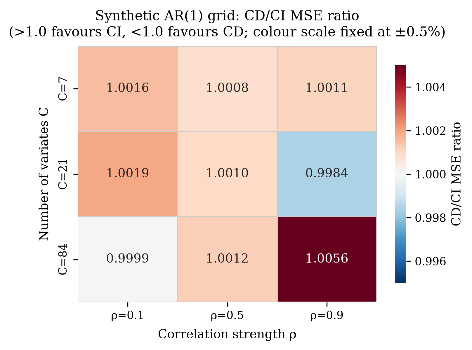
On the AR(1) grid the average difference was +0.13% of the CI error. Its seed-clustered 95% interval ran from −0.0023 to +0.0048 MSE.

The pooled detection half-width makes that stronger than “no difference found”. It came to about 0.62% of the CI error. Any uniform CD advantage bigger than that would have pushed the interval clear of zero. So it puts a measured ceiling on how big a hidden CD gain could be.

Heatmap of the CD/CI test-MSE ratio across the AR(1) grid by series count and correlation strength — **Accuracy parity.** AR(1) grid, CD/CI test-MSE ratio by series count and correlation. No cell departs from 1.0 by more than 0.56%, and the sign of the deviation flips across the grid.

Heatmap of the CD/CI test-MSE ratio across patch size and coupling strength, with grey cells where CD could not run — **Unequal feasibility.** Patch-resolution sweep, CD/CI ratio across patch size and lag-1 coupling. Every coloured cell is within 0.15% of 1.0; the grey cells at P = 2 are where CD exceeded T4 memory and could not run.

Why the signal went cold

To find the lowest error any model could possibly reach, I worked it out exactly from each family's equations, with no training involved. I did it twice, once giving the model all the series and once giving it each series' own history only. The gap between the two is the most a CD model could ever gain.

In the AR(1) and block-covariance families that gap is zero at every horizon. With a diagonal A, the best forecast h steps ahead is the same whether or not you see the other series:

x̂_t+h = φ^h x_t, error variance = 1 − φ^2h (z-scored units), for any ρ, C or block structure

The series are only linked by shocks that hit them at the same moment, and tomorrow's shock is unknowable from any series. At φ = 0.8 and h = 96 the term φ¹⁹² is about 2 × 10⁻¹⁹, so both floors sit at 1.0 to float64 precision: the forecast is the unconditional mean, and nothing can improve it.

The leader-follower family is the more interesting case. The leader does carry information about its followers, and that information fades with every step ahead. Unrolling the follower's equation h steps and taking expectations at time t gives

f̂_t+h = φ^h f_t + γ · h φ^h−1 · l_t

The second term is everything the leader's current value adds. Its weight hφ^h−1 rises from 1 at one step to a peak of 2.05 at four and five steps, which is where the paper's absolute gap peaks, then decays: 0.29 at 20 steps, 0.0009 at 50, and 6 × 10⁻⁸ at 96. The own-history forecaster is a steady-state Kalman filter that recovers part of l_t from the follower's own past, so the real CD advantage is smaller than this term suggests. The table shows the exact ceilings from the paper.

Forecast horizon	γ = 0.3	γ = 0.6	γ = 0.9
1 step ahead	9.8%	24.9%	39.6%
96 steps ahead, the last step scored	0	0	0

How to read it: each cell is the most CD could win over CI, as a share of the best CI error, for a given coupling strength γ. At 96 steps the two error floors match to float64 precision.

By the 96th step the leader's information has gone cold. CD can still mix the series, but at that step there is nothing left for it to serve. Inside the scored window the floors do separate at short steps, and the absolute gap peaks five steps ahead. That is where the next experiment belongs.

Checking the leftover gap

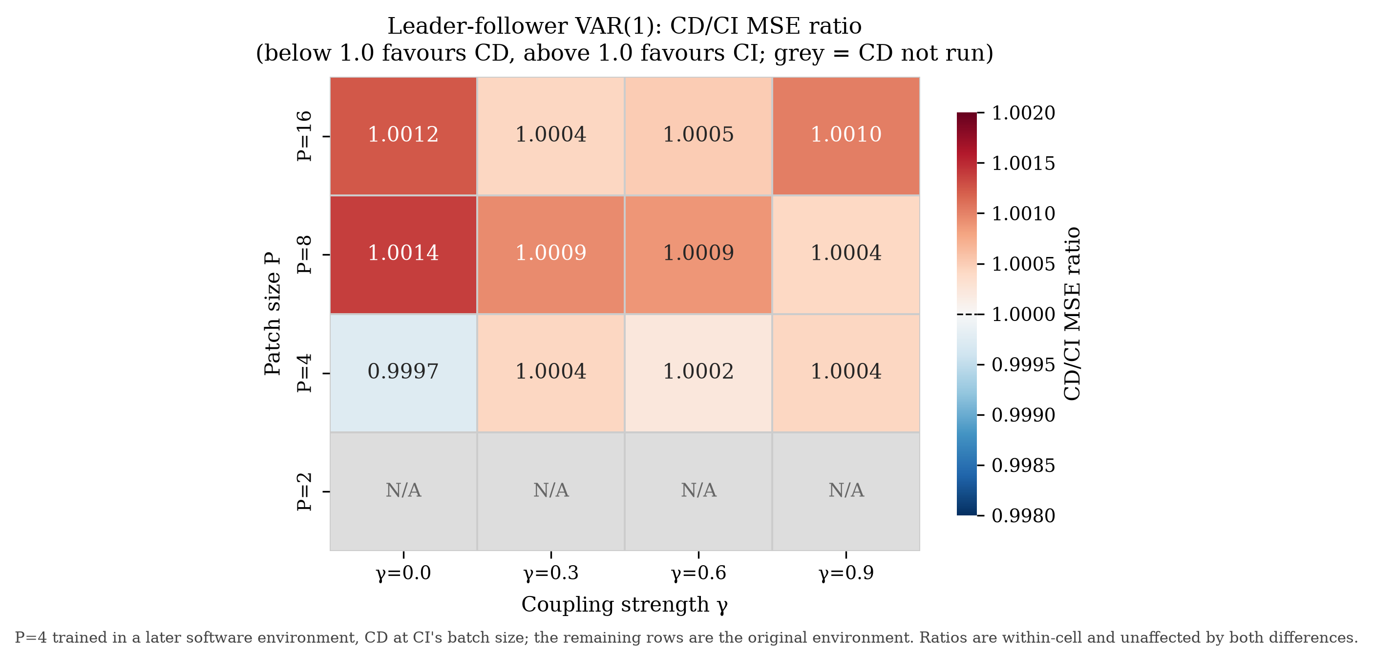
One pattern still needed checking. Under the original training setup, CD came out slightly worse than CI on the leader-follower data. The gap stayed inside the ±1% band but widened as the coupling got stronger. Before blaming the architecture, I tested two simpler explanations.

What was left

CD slightly behind CI on leader-follower data, gap growing with γ, still inside ±1%

Check 1 · optimisation exposure

Suspect: smaller feasible batches give CD many more updates per epoch, training it past its best↓Test: cap both designs at the same update budget↓The deficit does not survive the cap

Check 2 · interaction placement

Suspect: CD shares CI's per-series prediction head, and that head could be the bottleneck↓Test: a head that pools across series↓Ties CI at every γ

Both checks removed the pattern, and every variant stayed inside the ±1% band.

What it comes to

Correlated series aren't automatically informative series. What matters is whether seeing one series improves the forecast of another once you know the target's own past, at the horizon you need.

Two gates

That splits the decision into two gates that often get blurred.

Gate 1, information. Does another series improve the forecast once the target's own history is known, at the exact horizon that matters?
Gate 2, extraction. If that information exists, does the chosen cross-series architecture capture enough of it to repay its training, memory and operational cost?

At 96 steps, once a series' own history was known, the controlled processes offered no extra cross-series information. They failed the first gate, and the bill below shows how expensive flattened-token CD makes the second one to test.

The bill

Equal accuracy didn't make the two designs equal to run. Flattened-token CD needs smaller feasible batches, and smaller batches mean more gradient updates per epoch: updates = ⌈training windows / batch⌉, so at C = 84 CI's batch of 32 gives 233 updates per epoch and CD's batch of 1 gives 7,433, a 31.9× ratio before either model has learnt anything. In the two cells I compared, leader-follower at γ = 0.6 and the AR(1) grid at C = 84 and ρ = 0.9, CD used 5.6 and 15.6 times as many gradient updates to reach its validation-selected checkpoint. On ECL's 321 series, a CD epoch took about 956 seconds on a T4 against about 143 for CI at the same batch size. That's the 6.7× at the top.

CI≈143 s

CD≈956 s

Seconds per training epoch on ECL (321 series, batch 8, horizon 336, one T4 GPU)

The cost also turns into a hard limit as the problem grows. More series or finer patches mean a longer token sequence for CD. At 84 series its batch size drops to 1. At the finest patch size I tested, P = 2, it didn't fit in the T4's memory under non-fused attention and couldn't run at all.

Production forecasting usually means many signals, long lookback windows, or retraining across sites, regions or products. That is where this formulation gets expensive first. Equal accuracy at several times the compute changes the default.

House rules

I now work through three steps, in this order.

Ask the information question first. Is there a domain reason to expect another series to improve the forecast at the exact horizon that matters, once the target's own past is known?
Start from a strong CI baseline. When the answer is no or unclear, CI is the cheaper and more scalable default.
Make CD earn the upgrade. Compare it under a cost-aware protocol, fix the size of a meaningful gain in advance, and keep CD only if the gain clears it. Then keep measuring its cost.

A lead-lag relationship that matters one step ahead can be worth nothing 96 steps ahead. That's why the first question names a horizon. In practice the horizon comes from the decision the forecast feeds, and that makes it a product requirement.

An open kitchen

I wanted anyone to be able to check the numbers without taking my word for them. One command in the repository verifies every results file against a committed SHA-256 digest, runs the unit tests and recomputes every table and figure. It takes under a minute on a CPU. The scripts behind the paper's tables end in checks against the values the paper quotes or a committed reference file. An unexpected change gets checked at two levels, against the file digest and against the reported number. The version the paper cites is archived on Zenodo under a DOI, and so is every release from v1.2 on.

uv sync --all-groups
uv run python src/reproduce_all.py --tests

What I'm not claiming

Every finding depends on PatchTST's patch-based representation, the lookback windows I used and the flattened-token way of letting series interact. Designs that model cross-series structure differently, such as treating each series as a single token, may trade accuracy and cost differently. This study doesn't test them.

The null result also only covers the 96-step horizon. At short horizons the error floors separate, as the table above shows, and that regime is still open. The 1% band was set for step 96 and can't be carried below step 50 without restating it against those floors. On the two real datasets CD came out slightly behind. On ETTh1, under a matched update budget, CI kept a small but reliable edge, about 2.6% of its error pooled across horizons. On ECL, in a single-seed run, CD trailed by 5.6 to 7.6%.

Scope

I'm not claiming CD never helps. The one-step numbers above show where it could. Correlation alone isn't evidence of useful cross-series signal at your forecast horizon. Check for that signal first, then make the architecture repay its cost. A targeted CI–CD pilot on your own data usually costs less than adopting the more expensive design by default.

Paper, code and archive

Published in TMLR (2026) after one revision round with three reviewers.

Companion page: the experiment design, step by step
Paper and reviews: OpenReview
PDF
Code and data (MIT): GitHub. The version the paper cites is tag v1.0-tmlr.
Archive: Zenodo